Getting started with OGGM Edu: idealised glaciers#
OGGM Edu provides a simple way to experiment with glaciers on your computer. This is achieved by a high level interface to the different parts of the complex glacier model that is OGGM. You as a user will interact with a few objects that provide you with methods and attributes fitting for a glacier and the parts that make it up.
The goal of this notebook is to introduce you to OGGM Edu and how it can be used to simulate two idealised glaciers.
We begin by importing the classes that we need
from oggm_edu import MassBalance, GlacierBed, Glacier, GlacierCollection
The three main classes that we are going to use are the
GlacierBedMassBalanceGlacier
The GlacierBed provide an easy way to define the glacier bed while the MassBalance is used to define the mass balance of the glacier.
The Glacier then provide us with methods to progress and visualise the glacier and informative attributes.
To create a glacier we need to give it a bed and a mass balance.
First steps#
In our first experiment we want to create a glacier that is as simple as possible. This means a glacier bed with a constant slope and width and a simple mass balance. We begin with creating the bed of our glacier.
The glacier bed#
In its most simple form the glacier bed requires a top and bottom altitude, and a witdh.
# All arguments are specified in meters.
bed = GlacierBed(top=3400, bottom=1500, width=300)
# This gives us some statistics about the bed.
bed
| GlacierBed | |
|---|---|
| Bed type | Linear bed with a constant width |
| Top [m] | 3400 |
| Bottom [m] | 1500 |
| Width(s) [m] | [300] |
| Length [km] | 20.0 |
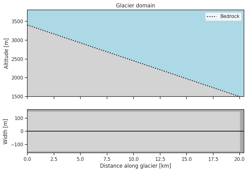
Let’s plot the bed to make sure that it looks like we expect.
The bed object has a built in method for this which provide us with a side and top-down view of the glacier domain.
bed.plot()
Note: if you want to change the plot size of all edu plots, you can try:
import oggm_edu
oggm_edu.set_params(figsize=(12, 9))
For finer control over the bed slope you can pass a single value to slopes during the creation
# This will give us a steeper bed compared to the default.
bed_with_slope = GlacierBed(top=3400, bottom=1500, width=300, slopes=25)
bed_with_slope.plot()

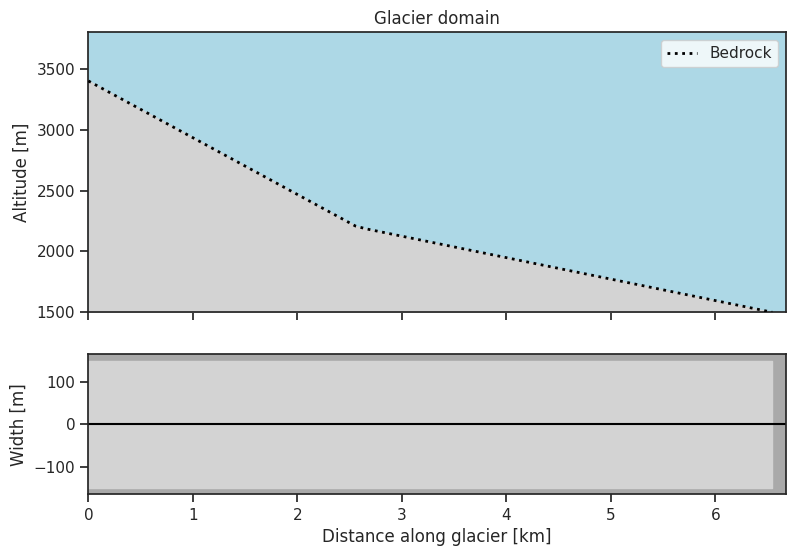
You can also pass a sequence of slope angles in slopes - for this you also need to specify the altitude spans of the sections with the slope_sections argument.
There should be one more entry in slope_sections compared to the entries in slopes.
The first and last value in slope_sections should match the top and bottom of the glacier.
# A bed with multiple slopes
bed_with_multiple_slopes = GlacierBed(top=3400, bottom=1500, width=300,
                                      slopes=[25, 10],
                                      # Slope sections are defined by altitude
                                      # pairs. Here we have two parirs.
                                      slope_sections=[3400, 2200, 1500])
bed_with_multiple_slopes.plot()
Mass balance#
For the glacier to grow it needs a mass balance model. The mass balance is responsible for adding snow and removing ice through melt on the glacier. In our case it will be a simple linear mass balance, meaning that it decreases linearly with altitude.
The mass balance is defined by the equilibrium line altitude (ELA) and the altitude gradient (in mm yr\(^{-1}\) m\(^{-1}\)). The ELA defines at what altitude the mass balance is zero and the altitude gradient how much the mass balance changes with altitude. More on this in upcoming notebooks!
We set the ELA of our glacier to 3000 meters and the altitude gradient to 4 mm yr\(^{-1}\) m\(^{-1}\).
mass_balance = MassBalance(ela=3000, gradient=4)
mass_balance
| MassBalance | |
|---|---|
| ELA [m] | 3000 |
| Original ELA [m] | 3000 |
| Temperature bias [C] | 0 |
| Gradient [mm/m/yr] | [4] |
Glacier initialisation#
We can now take our bed and the mass balance and create a glacier which we can then perform experiments on.
# Initialise the glacier
glacier = Glacier(bed=bed, mass_balance=mass_balance)
Similarly to the bed, we can get some statistics about the glacier by simply calling it. However since we just created the glacier, everything will be zero.
# Some statistics about the glacier
glacier
| Attribute | |
|---|---|
| Id | 1 |
| Type | Glacier |
| Age | 0 |
| Length [m] | 0.0 |
| Area [km2] | 0.0 |
| Volume [km3] | 0.0 |
| Max ice thickness [m] | 0.0 |
| Max ice velocity [m/yr] | None |
| AAR [%] | NaN |
| Response time [yrs] | NaN |
| Creep (Glen A) | 2.4e-24 |
| Basal sliding | 0 |
Progressing the glacier#
Now the glacier has all the ingredients needed to evolve.
Let’s first progress the glacier to year 1.
# We want to progress the glacier to year 1.
glacier.progress_to_year(1)
And let’s take a look at the glacier. As the bed, it has a in method for this.
glacier.plot()
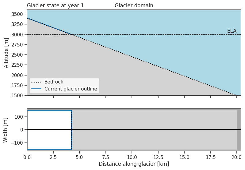
Here we can see that there is thin cover of ice from the top and 4 km down the glacier bed. So the glacier almost reaches the point where the bed intersects the ELA (~4 km). We can also take a look at some of statistics of the glacier again to get some more details:
glacier
| Attribute | |
|---|---|
| Id | 1 |
| Type | Glacier |
| Age | 1 |
| Length [m] | 4300.0 |
| Area [km2] | 1.29 |
| Volume [km3] | 0.00115 |
| Max ice thickness [m] | 1.782245 |
| Max ice velocity [m/yr] | 2.1045127747276928e-07 |
| AAR [%] | 97.674419 |
| Response time [yrs] | NaN |
| Creep (Glen A) | 2.4e-24 |
| Basal sliding | 0 |
From the statistics we can read that the glacier has a length of 4 km and covers an area of 1.2 km\(^2\). The glacier will grow considerably in the upcoming years, and the ice thickness should become apparent even in the altitude - distance plot. Let us progress the glacier to year 150 and take a look.
glacier.progress_to_year(150)
/usr/local/pyenv/versions/3.13.12/lib/python3.13/site-packages/oggm_edu/glacier.py:335: FutureWarning: In a future version of xarray the default value for data_vars will change from data_vars='all' to data_vars=None. This is likely to lead to different results when multiple datasets have matching variables with overlapping values. To opt in to new defaults and get rid of these warnings now use `set_options(use_new_combine_kwarg_defaults=True) or set data_vars explicitly.
  self._state_history = xr.combine_by_coords(
glacier.plot()
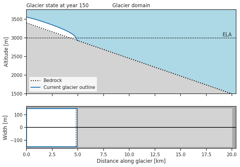
Now we can clearly see the difference between the surface of the glacier and the bedrock. Let’s print the same statistics about the glacier as before:
glacier
| Attribute | |
|---|---|
| Id | 1 |
| Type | Glacier |
| Age | 150 |
| Length [m] | 5000.0 |
| Area [km2] | 1.5 |
| Volume [km3] | 0.244588 |
| Max ice thickness [m] | 185.561606 |
| Max ice velocity [m/yr] | 58.101295324090245 |
| AAR [%] | 98.0 |
| Response time [yrs] | NaN |
| Creep (Glen A) | 2.4e-24 |
| Basal sliding | 0 |
The glacier length and area has increased by ~20% while the volume has increased by more than 1000%. This is because the glacier has to build enough mass (i.e. ice thickness) before it can begin to flow downhill and increase its length.
Note that the glacier is now 150 years old. If we try progressing the glacier to the same year again, nothing will happen. It evens gives us a warning.
glacier.progress_to_year(150)
/usr/local/pyenv/versions/3.13.12/lib/python3.13/site-packages/oggm_edu/glacier.py:559: UserWarning: Year has to be above the current age of the glacier. It is not possible to de-age the glacier. Geometry will remain the same.
  warnings.warn(msg)
We can easily progress the glacier even longer:
glacier.progress_to_year(500)
glacier.plot()
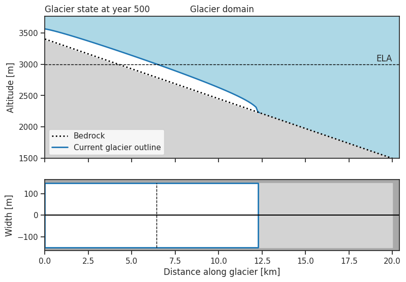
glacier
| Attribute | |
|---|---|
| Id | 1 |
| Type | Glacier |
| Age | 500 |
| Length [m] | 12300.0 |
| Area [km2] | 3.69 |
| Volume [km3] | 0.698493 |
| Max ice thickness [m] | 214.222348 |
| Max ice velocity [m/yr] | 64.3471902975956 |
| AAR [%] | 52.845528 |
| Response time [yrs] | NaN |
| Creep (Glen A) | 2.4e-24 |
| Basal sliding | 0 |
The glaciers has now grown considerably further down our made up mountain, well below the ELA.
It is important to note that the model can not progress back in time. Once at year 500, we can not de-age the glacier.
glacier.progress_to_year(450)
/usr/local/pyenv/versions/3.13.12/lib/python3.13/site-packages/oggm_edu/glacier.py:559: UserWarning: Year has to be above the current age of the glacier. It is not possible to de-age the glacier. Geometry will remain the same.
  warnings.warn(msg)
Let’s do the same with one of the glaciers with a non-linear bed profile!
# We create a new mass balance for this glacier.
mass_balance_2 = MassBalance(ela=2500, gradient=4)
# Initialise the glacier
glacier_multiple_slopes = Glacier(bed=bed_with_multiple_slopes,
                                  mass_balance=mass_balance_2)
# Progress the glacier
glacier_multiple_slopes.progress_to_year(400)
# And plot the glacier
glacier_multiple_slopes.plot()
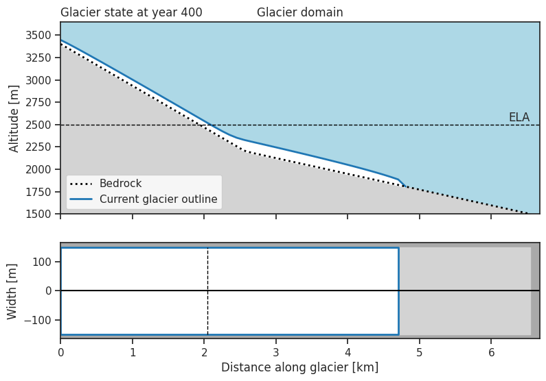
Glacier history#
This brings us to the glacier history.
This is just what it sounds like, a history of the length, volume and area of the glacier.
We can access the data through the .history attribute
glacier.history
<xarray.Dataset> Size: 48kB
Dimensions:           (time: 501)
Coordinates:
  * time              (time) float64 4kB 0.0 1.0 2.0 3.0 ... 498.0 499.0 500.0
    calendar_year     (time) int64 4kB 0 1 2 3 4 5 6 ... 495 496 497 498 499 500
    calendar_month    (time) int64 4kB 1 1 1 1 1 1 1 1 1 1 ... 1 1 1 1 1 1 1 1 1
    hydro_year        (time) int64 4kB 0 1 2 3 4 5 6 ... 495 496 497 498 499 500
    hydro_month       (time) int64 4kB 4 4 4 4 4 4 4 4 4 4 ... 4 4 4 4 4 4 4 4 4
Data variables:
    volume_m3         (time) float64 4kB 0.0 1.15e+06 ... 6.984e+08 6.985e+08
    volume_bsl_m3     (time) float64 4kB 0.0 0.0 0.0 0.0 0.0 ... 0.0 0.0 0.0 0.0
    volume_bwl_m3     (time) float64 4kB 0.0 0.0 0.0 0.0 0.0 ... 0.0 0.0 0.0 0.0
    area_m2           (time) float64 4kB 0.0 1.29e+06 ... 3.69e+06 3.69e+06
    length_m          (time) float64 4kB 0.0 4.3e+03 ... 1.23e+04 1.23e+04
    calving_m3        (time) float64 4kB 0.0 0.0 0.0 0.0 0.0 ... 0.0 0.0 0.0 0.0
    calving_rate_myr  (time) float64 4kB 0.0 0.0 0.0 0.0 0.0 ... 0.0 0.0 0.0 0.0
Attributes: (12/13)
    description:          OGGM model output
    oggm_version:         1.6.3.dev47+g61a0dd492
    calendar:             365-day no leap
    creation_date:        2026-03-09 20:56:37
    water_level:          0
    glen_a:               2.4e-24
    ...                   ...
    mb_model_class:       MassBalance
    mb_model_hemisphere:  nh
    mb_model_rho:         900.0
    mb_model_orig_ela_h:  3000
    mb_model_ela_h:       3000
mb_model_grad: 4And we can quickly visualise the history of the glacier with the .plot_history() method
glacier.plot_history()
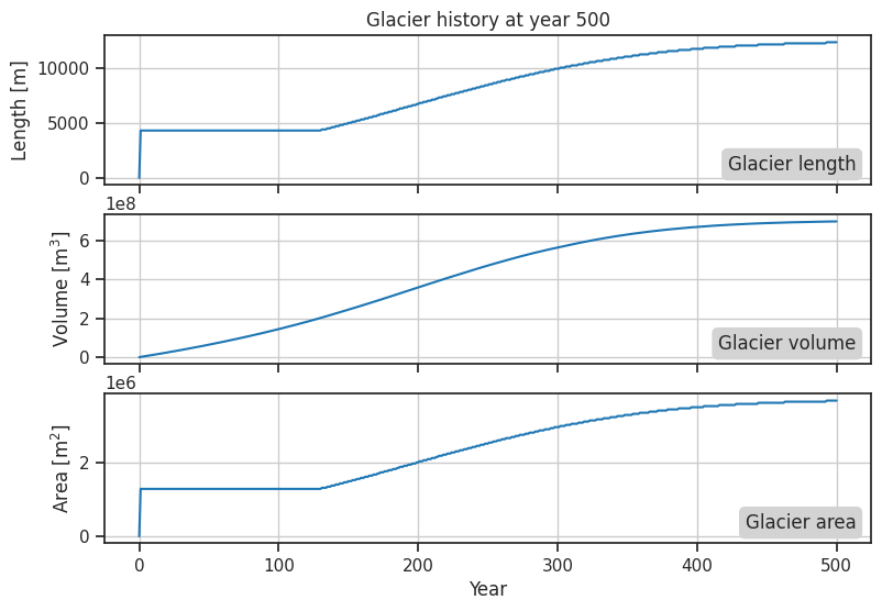
The glacier length and area has a step in the first year. This has to do with how OGGM internally deals with snow and ice, it does not differentiate between them. And since the mass balance is always positive above the ELA, any snowfall in the first year above the ELA will remain and be classified as part of the glacier, and contribute to the length and area.
This is why after the first year, the glacier’s length and area remains constant for a few years. In this initial stage, the ice is so thin that any flow bringing ice below the ELA will not be large enough to compensate for the high ablation rate, and any ice melts away.
When the ice thickness has increased enough for the ice flow to surpass the ablation rate below the ELA, the glacier length can begin to increase.
Equilibrium state#
After several centuries, the glacier reaches a balance with its climate.
This means that its length and volume won’t change anymore, as long as all physical parameters and the climate stay constant.
The Glacier has a method which progress the glacier to equilibrium .progress_to_equilibrium(), more on this in later notebooks.
A first experiment#
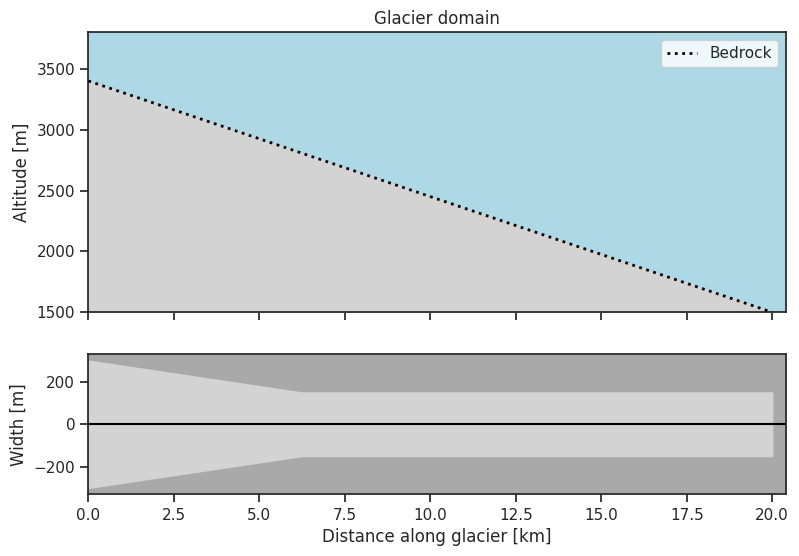
We have now seen how to setup a simple glacier and progress it to any year. Now we will move a little bit closer to reality and define a glacier with changing widths. Like many real glaciers the new glacier will be wider at the top (in the accumulation area) and have a constant width below the ELA.
We can achieve this by creating a new Bed and instead of specifying the top and bottom altitudes along with the width, we specify altitudes and widths in pairs:
wide_narrow_bed = GlacierBed(altitudes=[3400, 2800, 1500],
                             widths=[600, 300, 300])
wide_narrow_bed
| GlacierBed | |
|---|---|
| Bed type | Linear bed with a variable width |
| Top [m] | 3400 |
| Bottom [m] | 1500 |
| Width(s) [m] | [[600, 300, 300]] |
| Length [km] | 20.0 |
Here the first and last values in altitudes and widths correspond to the top/bottom altitude/width.
Any values in between will change the shape of the bed further.
wide_narrow_bed.plot()
We use the new bed to create a new glacier
wide_narrow_glacier = Glacier(bed=wide_narrow_bed,
                              mass_balance=mass_balance)
wide_narrow_glacier
| Attribute | |
|---|---|
| Id | 3 |
| Type | Glacier |
| Age | 0 |
| Length [m] | 0.0 |
| Area [km2] | 0.0 |
| Volume [km3] | 0.0 |
| Max ice thickness [m] | 0.0 |
| Max ice velocity [m/yr] | None |
| AAR [%] | NaN |
| Response time [yrs] | NaN |
| Creep (Glen A) | 2.4e-24 |
| Basal sliding | 0 |
We can now introduce the GlacierCollection.
This is a utility which can store multiple glaciers and can be used to easily compare and run experiments on multiple glaciers.
The GlacierCollection will be used extensively throughout these notebooks and its functionality will be explained further as we go along.
# We initialise a collection
collection = GlacierCollection()
# And then add the two glaciers available in this notebook.
collection.add([glacier, wide_narrow_glacier])
We can get a quick look at the collection by simply calling it
collection
| Id | Type | Age | Length [m] | Area [km2] | Volume [km3] | Max ice thickness [m] | Max ice velocity [m/yr] | AAR [%] | Response time [yrs] | ... | Basal sliding | Bed type | Top [m] | Bottom [m] | Width(s) [m] | Length [km] | ELA [m] | Original ELA [m] | Temperature bias [C] | Gradient [mm/m/yr] | |
|---|---|---|---|---|---|---|---|---|---|---|---|---|---|---|---|---|---|---|---|---|---|
| Glacier | |||||||||||||||||||||
| 1 | 1 | Glacier | 500 | 12300.0 | 3.69 | 0.698493 | 214.222348 | 64.34719 | 52.845528 | NaN | ... | 0 | Linear bed with a constant width | 3400 | 1500 | 300 | 20.0 | 3000 | 3000 | 0 | 4 |
| 2 | 3 | Glacier | 0 | 0.0 | 0.00 | 0.000000 | 0.000000 | None | NaN | NaN | ... | 0 | Linear bed with a variable width | 3400 | 1500 | [600, 300, 300] | 20.0 | 3000 | 3000 | 0 | 4 |
2 rows × 21 columns
Before plotting the glaciers in the collection, we can progress them to the same year with the .progress_to_year() method.
collection.progress_to_year(600)
We can then plot the collection
collection.plot()
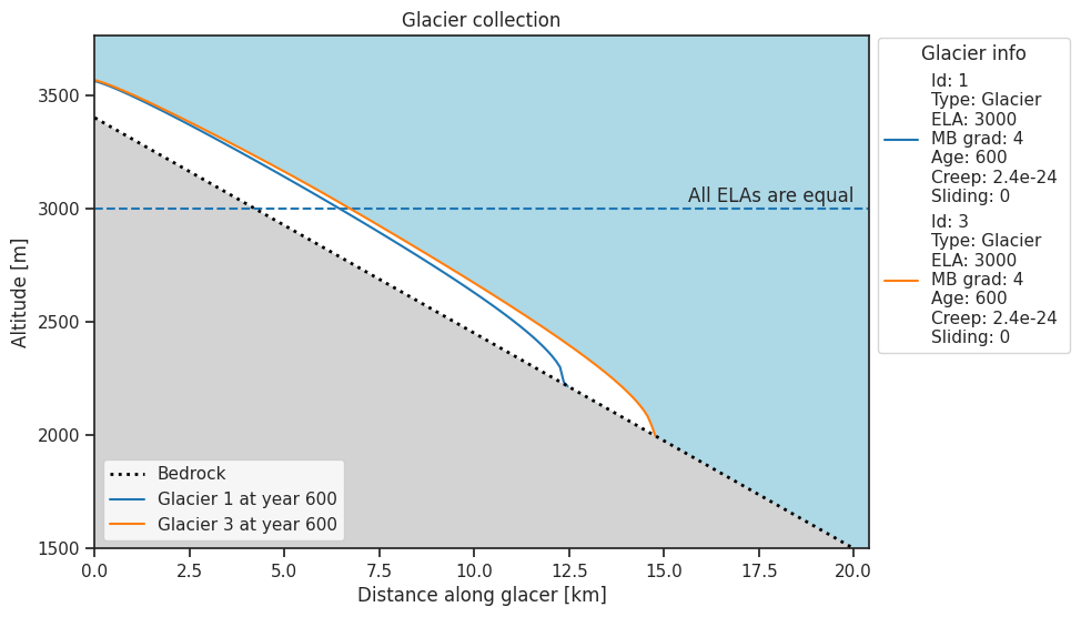
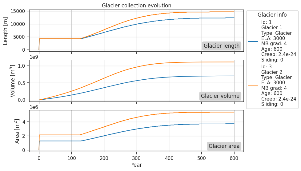
The glacier with a wider accumulation area is longer compared to the simple glacier area at year 600. With what you've learned so far in this notebook, can you come up with an explanation to why? Click for a hint
With a wider accumulation area the glacier mass above the ELA will increase quicker and the flow of ice to below the ELA will be larger compared to the glacier with a smaller accumulation area.Similarly to the glacier the collection has a method for easily plotting the histories of the held glaciers.
collection.plot_history()
