Glaciers as water resources: part 2 (projections) - OGGM versions pre 1.6#
Goals of this notebook:
run simulations using climate projections to explore the role of glaciers as water resources
Setting the scene: glacier runoff and “peak water”#
We strongly recommend to run Part 1 of this notebook before going on!
Setup#
import matplotlib.pyplot as plt
import seaborn as sns
sns.set_context('notebook')  # plot defaults
# Temporarily ignore warnings from shapely
import warnings
from shapely.errors import ShapelyDeprecationWarning
warnings.filterwarnings('ignore', category=ShapelyDeprecationWarning)
warnings.filterwarnings('ignore', message='Unpickling a shapely <2.0 geometry')
import xarray as xr
import salem
import numpy as np
import pandas as pd
import oggm.cfg
from oggm import utils, workflow, tasks, graphics
# OGGM options
oggm.cfg.initialize(logging_level='WARNING')
oggm.cfg.PATHS['working_dir'] = utils.gettempdir(dirname='WaterResources-Proj')
oggm.cfg.PARAMS['min_ice_thick_for_length'] = 1  # a glacier is when ice thicker than 1m
oggm.cfg.PARAMS['store_model_geometry'] = True
2023-08-27 22:05:37: oggm.cfg: Reading default parameters from the OGGM `params.cfg` configuration file.
2023-08-27 22:05:37: oggm.cfg: Multiprocessing switched OFF according to the parameter file.
2023-08-27 22:05:37: oggm.cfg: Multiprocessing: using all available processors (N=2)
2023-08-27 22:05:38: oggm.cfg: PARAMS['min_ice_thick_for_length'] changed from `0.0` to `1`.
2023-08-27 22:05:38: oggm.cfg: PARAMS['store_model_geometry'] changed from `False` to `True`.
Define the glacier we will play with#
For this notebook we use the Hintereisferner, Austria. Some other possibilities to play with:
Hintereisferner, Austria: RGI60-11.00897
Artesonraju, Peru: RGI60-16.02444
Rikha Samba, Nepal: RGI60-15.04847
Parlung No. 94, China: RGI60-15.11693
And virtually any glacier you can find the RGI Id from, e.g. in the GLIMS viewer! Large glaciers may need longer simulations to see changes though. For less uncertain calibration parameters, we also recommend to pick one of the many reference glaciers in this list, where we make sure that observations of mass-balance are better matched.
Let’s start with Hintereisferner first and you’ll be invited to try out your favorite glacier at the end of this notebook.
# Hintereisferner
rgi_id = 'RGI60-11.00897'
Preparing the glacier data#
This can take up to a few minutes on the first call because of the download of the required data:
# We pick the elevation-bands glaciers because they run a bit faster - but they create more step changes in the area outputs
base_url = 'https://cluster.klima.uni-bremen.de/~oggm/gdirs/oggm_v1.4/L3-L5_files/CRU/elev_bands/qc3/pcp2.5/no_match'
gdir = workflow.init_glacier_directories([rgi_id], from_prepro_level=5, prepro_border=80, prepro_base_url=base_url)[0]
2023-08-27 22:05:39: oggm.workflow: You seem to be using v1.4 directories with a more recent version of OGGM. While this is possible, be aware that some defaults parameters have changed. See the documentation for details: http://docs.oggm.org/en/stable/whats-new.html
2023-08-27 22:05:39: oggm.workflow: init_glacier_directories from prepro level 5 on 1 glaciers.
2023-08-27 22:05:39: oggm.workflow: Execute entity tasks [gdir_from_prepro] on 1 glaciers
Interactive glacier map#
A first glimpse on the glacier of interest.
Tip: You can use the mouse to pan and zoom in the map
# One interactive plot below requires Bokeh
# The rest of the notebook works without this dependency - comment if needed
import holoviews as hv
hv.extension('bokeh')
import geoviews as gv
import geoviews.tile_sources as gts

sh = salem.transform_geopandas(gdir.read_shapefile('outlines'))
(gv.Polygons(sh).opts(fill_color=None, color_index=None) *
 gts.tile_sources['EsriImagery'] * gts.tile_sources['StamenLabels']).opts(width=800, height=500, active_tools=['pan', 'wheel_zoom'])


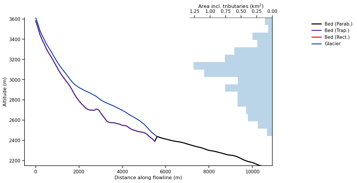
For OGGM, glaciers are “1.5” dimensional along their flowline:
fls = gdir.read_pickle('model_flowlines')
graphics.plot_modeloutput_section(fls);
“Commitment run”#
We are now ready to run our first simulation. This is a so called “commitment run”: how much ice loss is “already committed” for this glacier, even if climate change would stop today? This is a useful but purely theoretical experiment: climate change won’t stop today, unfortunately. To learn more about committed mass-loss at the global scale, read Marzeion et al., 2018.
Here, we run a simulation for 100 years with a constant climate based on the last 11 years:
# file identifier where the model output is saved
file_id = '_ct'

# We are using the task run_with_hydro to store hydrological outputs along with the usual glaciological outputs
tasks.run_with_hydro(gdir,
                     run_task=tasks.run_constant_climate,  # which climate? See below for other examples
                     nyears=100,  # length of the simulation
                     y0=2014, halfsize=5,  # For the constant climate, period over which the climate is taken from
                     store_monthly_hydro=True,  # Monthly ouptuts provide additional information
                     output_filesuffix=file_id);  # an identifier for the output file to read it later
2023-08-27 22:05:46: oggm.core.flowline: FileNotFoundError occurred during task run_constant_climate_ct on RGI60-11.00897: [Errno 2] No such file or directory: '/tmp/OGGM/WaterResources-Proj/per_glacier/RGI60-11/RGI60-11.00/RGI60-11.00897/mb_calib.json'
2023-08-27 22:05:46: oggm.core.flowline: FileNotFoundError occurred during task run_with_hydro_ct on RGI60-11.00897: [Errno 2] No such file or directory: '/tmp/OGGM/WaterResources-Proj/per_glacier/RGI60-11/RGI60-11.00/RGI60-11.00897/mb_calib.json'
---------------------------------------------------------------------------
FileNotFoundError                         Traceback (most recent call last)
Cell In[10], line 5
      2 file_id = '_ct'
      4 # We are using the task run_with_hydro to store hydrological outputs along with the usual glaciological outputs
----> 5 tasks.run_with_hydro(gdir,
      6                      run_task=tasks.run_constant_climate,  # which climate? See below for other examples
      7                      nyears=100,  # length of the simulation
      8                      y0=2014, halfsize=5,  # For the constant climate, period over which the climate is taken from
      9                      store_monthly_hydro=True,  # Monthly ouptuts provide additional information
     10                      output_filesuffix=file_id);  # an identifier for the output file to read it later

File /usr/local/pyenv/versions/3.10.12/lib/python3.10/site-packages/oggm/utils/_workflow.py:492, in entity_task.__call__.<locals>._entity_task(gdir, reset, print_log, return_value, continue_on_error, add_to_log_file, **kwargs)
    490     signal.alarm(cfg.PARAMS['task_timeout'])
    491 ex_t = time.time()
--> 492 out = task_func(gdir, **kwargs)
    493 ex_t = time.time() - ex_t
    494 if cfg.PARAMS['task_timeout'] > 0:

File /usr/local/pyenv/versions/3.10.12/lib/python3.10/site-packages/oggm/core/flowline.py:3759, in run_with_hydro(gdir, run_task, store_monthly_hydro, fixed_geometry_spinup_yr, ref_area_from_y0, ref_area_yr, ref_geometry_filesuffix, **kwargs)
   3756 if fixed_geometry_spinup_yr is not None:
   3757     kwargs['fixed_geometry_spinup_yr'] = fixed_geometry_spinup_yr
-> 3759 out = run_task(gdir, **kwargs)
   3761 if out is None:
   3762     raise InvalidWorkflowError('The run task ({}) did not run '
   3763                                'successfully.'.format(run_task.__name__))

File /usr/local/pyenv/versions/3.10.12/lib/python3.10/site-packages/oggm/utils/_workflow.py:492, in entity_task.__call__.<locals>._entity_task(gdir, reset, print_log, return_value, continue_on_error, add_to_log_file, **kwargs)
    490     signal.alarm(cfg.PARAMS['task_timeout'])
    491 ex_t = time.time()
--> 492 out = task_func(gdir, **kwargs)
    493 ex_t = time.time() - ex_t
    494 if cfg.PARAMS['task_timeout'] > 0:

File /usr/local/pyenv/versions/3.10.12/lib/python3.10/site-packages/oggm/core/flowline.py:3513, in run_constant_climate(gdir, nyears, y0, halfsize, ys, ye, bias, temperature_bias, precipitation_factor, store_monthly_step, store_model_geometry, store_fl_diagnostics, init_model_filesuffix, init_model_yr, output_filesuffix, climate_filename, mb_model_class, climate_input_filesuffix, init_model_fls, zero_initial_glacier, **kwargs)
   3428 @entity_task(log)
   3429 def run_constant_climate(gdir, nyears=1000, y0=None, halfsize=15,
   3430                          ys=None, ye=None,
   (...)
   3443                          zero_initial_glacier=False,
   3444                          **kwargs):
   3445     """Runs the constant mass balance model for a given number of years.
   3446
   3447     This will initialize a
   (...)
   3510         kwargs to pass to the FluxBasedModel instance
   3511     """
-> 3513     mb_model = MultipleFlowlineMassBalance(gdir,
   3514                                            mb_model_class=partial(
   3515                                                ConstantMassBalance,
   3516                                                mb_model_class=mb_model_class),
   3517                                            y0=y0, halfsize=halfsize,
   3518                                            bias=bias,
   3519                                            filename=climate_filename,
   3520                                            input_filesuffix=climate_input_filesuffix)
   3522     if temperature_bias is not None:
   3523         mb_model.temp_bias += temperature_bias

File /usr/local/pyenv/versions/3.10.12/lib/python3.10/site-packages/oggm/core/massbalance.py:1199, in MultipleFlowlineMassBalance.__init__(self, gdir, fls, mb_model_class, use_inversion_flowlines, input_filesuffix, **kwargs)
   1195     else:
   1196         rgi_filesuffix = input_filesuffix
   1198     self.flowline_mb_models.append(
-> 1199         mb_model_class(gdir, input_filesuffix=rgi_filesuffix,
   1200                        **kwargs))
   1202 self.valid_bounds = self.flowline_mb_models[-1].valid_bounds
   1203 self.hemisphere = gdir.hemisphere

File /usr/local/pyenv/versions/3.10.12/lib/python3.10/site-packages/oggm/core/massbalance.py:712, in ConstantMassBalance.__init__(self, gdir, mb_model_class, y0, halfsize, **kwargs)
    695 """Initialize
    696
    697 Parameters
   (...)
    708     keyword arguments to pass to the mb_model_class
    709 """
    711 super().__init__()
--> 712 self.mbmod = mb_model_class(gdir,
    713                             **kwargs)
    715 if y0 is None:
    716     raise InvalidParamsError('Please set `y0` explicitly')

File /usr/local/pyenv/versions/3.10.12/lib/python3.10/site-packages/oggm/core/massbalance.py:384, in MonthlyTIModel.__init__(self, gdir, filename, input_filesuffix, fl_id, melt_f, temp_bias, prcp_fac, bias, ys, ye, repeat, check_calib_params)
    381 self.gdir = gdir
    383 if melt_f is None:
--> 384     melt_f = self.calib_params['melt_f']
    386 if temp_bias is None:
    387     temp_bias = self.calib_params['temp_bias']

File /usr/local/pyenv/versions/3.10.12/lib/python3.10/site-packages/oggm/utils/_workflow.py:299, in lazy_property.<locals>._lazy_property(self)
    295 @property
    296 @wraps(fn)
    297 def _lazy_property(self):
    298     if not hasattr(self, attr_name):
--> 299         setattr(self, attr_name, fn(self))
    300     return getattr(self, attr_name)

File /usr/local/pyenv/versions/3.10.12/lib/python3.10/site-packages/oggm/core/massbalance.py:546, in MonthlyTIModel.calib_params(self)
    543 @lazy_property
    544 def calib_params(self):
    545     if self.fl_id is None:
--> 546         return self.gdir.read_json('mb_calib')
    547     else:
    548         try:

File /usr/local/pyenv/versions/3.10.12/lib/python3.10/site-packages/oggm/utils/_workflow.py:3222, in GlacierDirectory.read_json(self, filename, filesuffix, allow_empty)
   3220         out = {}
   3221 else:
-> 3222     with open(fp, 'r') as f:
   3223         out = json.load(f)
   3224 return out

FileNotFoundError: [Errno 2] No such file or directory: '/tmp/OGGM/WaterResources-Proj/per_glacier/RGI60-11/RGI60-11.00/RGI60-11.00897/mb_calib.json'
Then we can take a look at the output:
with xr.open_dataset(gdir.get_filepath('model_diagnostics', filesuffix=file_id)) as ds:
    # The last step of hydrological output is NaN (we can't compute it for this year)
    ds = ds.isel(time=slice(0, -1)).load()
There are plenty of variables in this dataset! We can list them with:
ds
Tip: you can click on a variable and show it’s attribute with the “page” button on the right.
The time and month_2d variables are coordinates, and the other variables are either provided as additional information (e.g. calendar_month, we will get back to this), or they are providing the actual data. For instance, we can plot the annual evolution of the volume and length of our glacier:
fig, axs = plt.subplots(nrows=2, figsize=(10, 7), sharex=True)
ds.volume_m3.plot(ax=axs[0]);
ds.length_m.plot(ax=axs[1]);
axs[0].set_xlabel(''); axs[0].set_title(f'{rgi_id}'); axs[1].set_xlabel('Years');
The glacier length and volume decrease during the first ~40 years of the simulation - this is the glacier retreat phase. Afterwards, both length and volume oscillate around a more or less constant value indicating that the glacier has reached equilibrium. The difference between the starting volume and the equilibrium volume is called the committed mass loss. It can be quite high in the Alps, and depends on many factors (such as glacier size, location, and the reference climate period),
Annual runoff#
As glaciers retreat, they contribute to sea-level rise (visit the World Glaciers Explorer OGGM-Edu app for more information!). This is not what we are interested in here. Indeed, they will also have important local impacts: in this notebook, we will have a look at their impact on streamflow.
Let’s take a look at some of the hydrological outputs computed by OGGM. We start by creating a pandas DataFrame of all “1D” (annual) variables:
sel_vars = [v for v in ds.variables if 'month_2d' not in ds[v].dims]
df_annual = ds[sel_vars].to_dataframe()
Then we can select the hydrological varialbes and sum them to get the total annual runoff:
# Select only the runoff variables
runoff_vars = ['melt_off_glacier', 'melt_on_glacier', 'liq_prcp_off_glacier', 'liq_prcp_on_glacier']
# Convert them to megatonnes (instead of kg)
df_runoff = df_annual[runoff_vars] * 1e-9
fig, ax = plt.subplots(figsize=(10, 3.5), sharex=True)
df_runoff.sum(axis=1).plot(ax=ax);
plt.ylabel('Mt'); plt.xlabel('Years'); plt.title(f'Total annual runoff for {rgi_id}');
The hydrological variables are computed on the largest possible area that was covered by glacier ice during the simulation. This is equivalent to the runoff that would be measured at a fixed-gauge hydrological station at the glacier terminus.
The total annual runoff consists of the following components:
melt off-glacier: snow melt on areas that are now glacier free (i.e. 0 in the year of largest glacier extent, in this example at the start of the simulation)
melt on-glacier: ice + seasonal snow melt on the glacier
liquid precipitaton on- and off-glacier (the latter being zero at the year of largest glacial extent, in this example at start of the simulation)
f, ax = plt.subplots(figsize=(10, 6));
df_runoff.plot.area(ax=ax, color=sns.color_palette("rocket")); plt.xlabel('Years'); plt.ylabel('Runoff (Mt)'); plt.title(rgi_id);
Before we continue, let’s remember ourselves the expected contribution of glaciers to runoff.
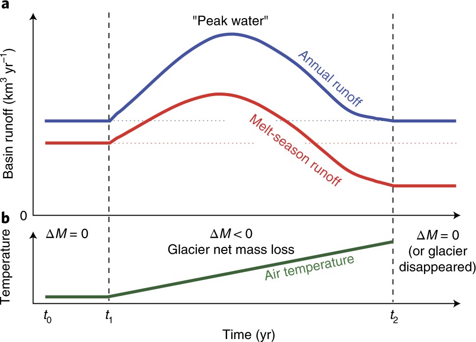
Graphic from Huss & Hock (2018)
Questions to explore:
where approximately on this graph is the studied glacier?
can you explain the relative contribution of each component, based on the previous notebook?
The total runoff out of a glacier basin is the sum of the four contributions above. To show that the glacier total contribution is indeed zero (\(\Delta M = 0\)) when in equilibrium, we can compute it from the glacier mass change:
glacier_mass = ds.volume_m3.to_series() * oggm.cfg.PARAMS['ice_density'] * 1e-9  # In Megatonnes, Mt

glacier_mass.diff().plot()
plt.axhline(y=0, color='k', ls=':')
plt.ylabel('Annual glacier mass change (Mt yr$^{-1}$)')
plt.xlabel('Years'); plt.title('Glacier contribution to annual runoff');
Note that this doesn’t mean that ice is not melting! At equilibrium, this means that the ice that melts each year over the glacier is replaced by snowfall in the accumulation area of the glacier. This illustrates well that glaciers in equilibrium are not net water resources on the annual average: in the course of the year they gain as much mass as they release.
Monthly runoff#
The “2D” variables contain the same data but at monthly resolution, with the dimension (time, month). For example, runoff can be computed the same way:
# Select only the runoff variables and convert them to megatonnes (instead of kg)
monthly_runoff = (ds['melt_off_glacier_monthly'] + ds['melt_on_glacier_monthly'] +
                  ds['liq_prcp_off_glacier_monthly'] + ds['liq_prcp_on_glacier_monthly'])
monthly_runoff *= 1e-9
monthly_runoff.clip(0).plot(cmap='Blues', cbar_kwargs={'label': 'Mt'}); plt.xlabel('Months'); plt.ylabel('Years');
But be aware, something is a bit wrong with this: the coordinates are hydrological months - let’s make this better:
# This should work in both hemispheres maybe?
ds_roll = ds.roll(month_2d=ds['calendar_month_2d'].data[0] - 1, roll_coords=True)
ds_roll['month_2d'] = ds_roll['calendar_month_2d']

# Select only the runoff variables and convert them to megatonnes (instead of kg)
monthly_runoff = (ds_roll['melt_off_glacier_monthly'] + ds_roll['melt_on_glacier_monthly'] +
                  ds_roll['liq_prcp_off_glacier_monthly'] + ds_roll['liq_prcp_on_glacier_monthly'])
monthly_runoff *= 1e-9
monthly_runoff.clip(0).plot(cmap='Blues', cbar_kwargs={'label': 'Mt'}); plt.xlabel('Months'); plt.ylabel('Years');
As we can see, the runoff is approximately zero during the winter months, while relatively high during the summer months. This implies that the glacier is a source of water in the summer when it releases the water accumulated in the winter.
The annual cycle changes as the glacier retreats:
monthly_runoff.sel(time=[0, 30, 99]).plot(hue='time');
plt.title('Annual cycle');
plt.xlabel('Month');
plt.ylabel('Runoff (Mt)');
Not only does the total runoff during the summer months decrease as the simulation progresses, the month of maximum runoff is also shifted to earlier in the summer.
CMIP5 projection runs#
You have now learned how to simulate and analyse a specific glacier under a constant climate. We will now take this a step further and simulate two different glaciers, located in different climatic regions, forced with CMIP5 climate projections.
We begin by initializing the glacier directories:
# We keep Hintereisferner from earlier, but also add a new glacier
rgi_ids = [rgi_id, 'RGI60-15.02420']
gdirs = workflow.init_glacier_directories(rgi_ids, from_prepro_level=5, prepro_border=80, prepro_base_url=base_url)
gdirs now contain two glaciers, one in Central Europe and one in the Eastern Himlayas:
gdirs
We can take a quick look at the new glacier:
sh = salem.transform_geopandas(gdirs[1].read_shapefile('outlines'))
(gv.Polygons(sh).opts(fill_color=None, color_index=None) *
 gts.tile_sources['EsriImagery'] * gts.tile_sources['StamenLabels']).opts(width=800, height=500, active_tools=['pan', 'wheel_zoom'])
Climate downscaling#
Before we run our simulation we have to process the climate data for the glaicer i.e. downscale it: (This can take some time)
from oggm.shop import gcm_climate
bp = 'https://cluster.klima.uni-bremen.de/~oggm/cmip5-ng/pr/pr_mon_CCSM4_{}_r1i1p1_g025.nc'
bt = 'https://cluster.klima.uni-bremen.de/~oggm/cmip5-ng/tas/tas_mon_CCSM4_{}_r1i1p1_g025.nc'
for rcp in ['rcp26', 'rcp45', 'rcp60', 'rcp85']:
    # Download the files
    ft = utils.file_downloader(bt.format(rcp))
    fp = utils.file_downloader(bp.format(rcp))
    workflow.execute_entity_task(gcm_climate.process_cmip_data, gdirs,
                                 # Name file to recognize it later
                                 filesuffix='_CCSM4_{}'.format(rcp),
                                 # temperature projections
                                 fpath_temp=ft,
                                 # precip projections
                                 fpath_precip=fp,
                                 );
Projection run#
With the downscaling complete, we can run the forced simulations:
for rcp in ['rcp26', 'rcp45', 'rcp60', 'rcp85']:
    rid = '_CCSM4_{}'.format(rcp)
    workflow.execute_entity_task(tasks.run_with_hydro, gdirs,
                                 run_task=tasks.run_from_climate_data, ys=2020,
                                 # use gcm_data, not climate_historical
                                 climate_filename='gcm_data',
                                 # use the chosen scenario
                                 climate_input_filesuffix=rid,
                                 # this is important! Start from 2020 glacier
                                 init_model_filesuffix='_historical',
                                 # recognize the run for later
                                 output_filesuffix=rid,
                                 # add monthly diagnostics
                                 store_monthly_hydro=True);
# Create the figure
f, ax = plt.subplots(figsize=(18, 7), sharex=True)
# Loop over all scenarios
for i, rcp in enumerate(['rcp26', 'rcp45', 'rcp60', 'rcp85']):
    file_id = f'_CCSM4_{rcp}'
    # Open the data, gdirs[0] correspond to Hintereisferner.
    with xr.open_dataset(gdirs[0].get_filepath('model_diagnostics', filesuffix=file_id)) as ds:
        # Load the data into a dataframe
        ds = ds.isel(time=slice(0, -1)).load()

    # Select annual variables
    sel_vars = [v for v in ds.variables if 'month_2d' not in ds[v].dims]
    # And create a dataframe
    df_annual = ds[sel_vars].to_dataframe()

    # Select the variables relevant for runoff.
    runoff_vars = ['melt_off_glacier', 'melt_on_glacier', 'liq_prcp_off_glacier', 'liq_prcp_on_glacier']
    # Convert to mega tonnes instead of kg.
    df_runoff = df_annual[runoff_vars].clip(0) * 1e-9
    # Sum the variables each year "axis=1", take the 11 year rolling mean and plot it.
    df_roll = df_runoff.sum(axis=1).rolling(window=11, center=True).mean()
    df_roll.plot(ax=ax, label=rcp, color=sns.color_palette("rocket")[i])

ax.set_ylabel('Annual runoff (Mt)'); ax.set_xlabel('Year'); plt.title(gdirs[0].rgi_id); plt.legend();
For Hintereisferner, runoff continues to decrease throughout the 21st-century for all scenarios, indicating that peak water has already been reached sometime in the past. This is the case for many European glaciers. What about our unnamed glacier in the Himalayas?
# Create the figure
f, ax = plt.subplots(figsize=(18, 7), sharex=True)
# Loop over all scenarios
for i, rcp in enumerate(['rcp26', 'rcp45', 'rcp60', 'rcp85']):
    file_id = f'_CCSM4_{rcp}'
    # Open the data, gdirs[1] correspond to the unnamed glacier.
    with xr.open_dataset(gdirs[1].get_filepath('model_diagnostics', filesuffix=file_id)) as ds:
        # Load the data into a dataframe
        ds = ds.isel(time=slice(0, -1)).load()

    # Select annual variables
    sel_vars = [v for v in ds.variables if 'month_2d' not in ds[v].dims]
    # And create a dataframe
    df_annual = ds[sel_vars].to_dataframe()

    # Select the variables relevant for runoff.
    runoff_vars = ['melt_off_glacier', 'melt_on_glacier',
                   'liq_prcp_off_glacier', 'liq_prcp_on_glacier']
    # Convert to mega tonnes instead of kg.
    df_runoff = df_annual[runoff_vars].clip(0) * 1e-9
    # Sum the variables each year "axis=1", take the 11 year rolling mean and plot it.
    df_roll = df_runoff.sum(axis=1).rolling(window=11, center=True).mean()
    df_roll.plot(ax=ax, label=rcp, color=sns.color_palette("rocket")[i])

ax.set_ylabel('Annual runoff (Mt)'); ax.set_xlabel('Year'); plt.title(gdirs[1].rgi_id); plt.legend();
Unlike for Hintereisferner, these projections indicate that the annual runoff will increase in all the scenarios for the first half of the century. The higher RCP scenarios can reach peak water later in the century, since the excess melt can continue to increase. For the lower RCP scenarios on the other hand, the glacier might be approaching a new equilibirum, which reduces the runoff earlier in the century (Rounce et. al., 2020). After peak water is reached (RCP2.6: ~2055, RCP8.5: ~2070 in these projections), the annual runoff begins to decrease. This decrease occurs because the shrinking glacier is no longer able to support the high levels of melt.
Another projection run with temperature bias, or precipitation?#
TODO: include something about how temperature bias affect the size of the glacier and the meltwater output.
Take home points#
Glaciers in equilibrium are not net water resources: they gain as much mass as they release over a year.
However, they have a seasonal buffer role: they release water during the melt months.
The size of a glacier has an influence on the water availability downstream during the dry season. The impact is most important if the (warm) melt season coincides with the dry season (see Kaser et al., 2010).
When glaciers melt, they become net water resources over the year. “Peak water” is the point in time when glacier melt supply reaches its maximum, i.e. when the maximum runoff occurs.
References#
Kaser, G., Großhauser, M., and Marzeion, B.: Contribution potential of glaciers to water availability in different climate regimes, PNAS, 07 (47) 20223-20227, doi:10.1073/pnas.1008162107, 2010
Huss, M. and Hock, R.: Global-scale hydrological response to future glacier mass loss, Nat. Clim. Chang., 8(2), 135–140, doi:10.1038/s41558-017-0049-x, 2018.
Marzeion, B., Kaser, G., Maussion, F. and Champollion, N.: Limited influence of climate change mitigation on short-term glacier mass loss, Nat. Clim. Chang., 8, doi:10.1038/s41558-018-0093-1, 2018.
Rounce, D. R., Hock, R., McNabb, R. W., Millan, R., Sommer, C., Braun, M. H., Malz, P., Maussion, F., Mouginot, J., Seehaus, T. C. and Shean, D. E.: Distributed global debris thickness estimates reveal debris significantly impacts glacier mass balance, Geophys. Res. Lett., doi:10.1029/2020GL091311, 2021.
What’s next?#
Back to the table of contents